设置

import numpy as np
import tensorflow as tf
from tensorflow import keras

介绍

迁移学习是在一个特定的问题上学到的特征，并在新的类似问题上加以利用。例如，来自已学会识别浣熊的模型的特征可能对启动旨在识别狸小动物的模型很有用。

迁移学习通常是针对数据集数据太少而无法从头训练完整模型的任务完成的。

在深度学习中，迁移学习最常见的体现是以下问题：

1. 从先前训练过的模型中获取图层。
2. 冻结它们，以免在以后的训练中破坏它们包含的任何信息。
3. 在冻结层的顶部添加一些新的可训练层。他们将学习将旧功能转变为对新数据集的预测。
4. 在数据集上训练新图层。
   最后一个可选步骤是微调（fine-tuning），包括取消冻结上面获得的整个模型（或模型的一部分），并以非常低的学习率对新数据进行重新训练。通过将预训练的功能逐步适应新数据，可以潜在地实现有意义的改进。

首先，我们将详细介绍Keras可训练的API，它是大多数迁移学习和微调工作流的基础。

然后，我们将通过在ImageNet数据集上进行预训练的模型，然后在Kaggle“猫与狗”分类数据集上对其进行重新训练，来演示典型的工作流程。

改编自Python深度学习和2016年博客文章“使用很少的数据构建强大的图像分类模型”。

冻结层：了解可训练的属性

图层和模型具有三个权重属性：

• weights 是该层的所有权重变量的列表。
• trainable_weights是旨在（通过梯度下降）进行更新以最大程度地减少训练过程中的损失的列表。
• non_trainable_weights是不适合训练的列表。 通常，它们在正向传递期间由模型更新。
  示例：密集层具有2个可训练的权重（内核和偏差）

layer = keras.layers.Dense(3)
layer.build((None, 4))  # Create the weights

print("weights:", len(layer.weights))
print("trainable_weights:", len(layer.trainable_weights))
print("non_trainable_weights:", len(layer.non_trainable_weights))

weights: 2
trainable_weights: 2
non_trainable_weights: 0

通常，所有权重（weights） 都是可训练的权重。 唯一具有不可调整权重的内置层是BatchNormalization层。 它使用不可训练的权重来跟踪训练期间其输入的均值和方差。 要了解如何在自己的自定义图层中使用不可训练的权重，请参阅从头开始编写新图层的指南。

示例：BatchNormalization图层具有2个可训练的权重和2个不可训练的权重

layer = keras.layers.BatchNormalization()
layer.build((None, 4))  # Create the weights

print("weights:", len(layer.weights))
print("trainable_weights:", len(layer.trainable_weights))
print("non_trainable_weights:", len(layer.non_trainable_weights))

weights: 4
trainable_weights: 2
non_trainable_weights: 2

图层和模型还具有可训练的布尔属性。 其值可以更改。 将layer.trainable设置为False会将图层的所有权重从可训练变为不可训练。 这称为“冻结”层：冻结层的状态在训练期间不会更新（无论是使用fit（）进行训练，还是使用依赖于trainable_weights来应用梯度更新的任何自定义循环进行训练）。

例子: 设置trainable 为 False

layer = keras.layers.Dense(3)
layer.build((None, 4))  # Create the weights
layer.trainable = False  # Freeze the layer

print("weights:", len(layer.weights))
print("trainable_weights:", len(layer.trainable_weights))
print("non_trainable_weights:", len(layer.non_trainable_weights))

weights: 2
trainable_weights: 0
non_trainable_weights: 2
当可训练的重量变得不可训练时，其值将在训练期间不再更新。

# Make a model with 2 layers
layer1 = keras.layers.Dense(3, activation="relu")
layer2 = keras.layers.Dense(3, activation="sigmoid")
model = keras.Sequential([keras.Input(shape=(3,)), layer1, layer2])

# Freeze the first layer
layer1.trainable = False

# Keep a copy of the weights of layer1 for later reference
initial_layer1_weights_values = layer1.get_weights()

# Train the model
model.compile(optimizer="adam", loss="mse")
model.fit(np.random.random((2, 3)), np.random.random((2, 3)))

# Check that the weights of layer1 have not changed during training
final_layer1_weights_values = layer1.get_weights()
np.testing.assert_allclose(
    initial_layer1_weights_values[0], final_layer1_weights_values[0]
)
np.testing.assert_allclose(
    initial_layer1_weights_values[1], final_layer1_weights_values[1]

1/1 [==============================] - 0s 1ms/step - loss: 0.0846
不要将layer.trainable属性与layer .__ call __（）中的训练变量混淆（该参数控制该层是应该以推理模式还是训练模式运行其前向传递）。 有关更多信息，请参见Keras FAQ。

可训练属性的递归设置

如果你在模型或具有子图层的任何图层上设置rainable = False，则所有子图层也将变为不可训练。

例子：

inner_model = keras.Sequential(
    [
        keras.Input(shape=(3,)),
        keras.layers.Dense(3, activation="relu"),
        keras.layers.Dense(3, activation="relu"),
    ]
)

model = keras.Sequential(
    [keras.Input(shape=(3,)), inner_model, keras.layers.Dense(3, activation="sigmoid"),]
)

model.trainable = False  # Freeze the outer model

assert inner_model.trainable == False  # All layers in `model` are now frozen
assert inner_model.layers[0].trainable == False  # `trainable` is propagated recursively

典型的迁移学习工作流程

这使我们了解如何在Keras中实现典型的转学学习工作流程：

1. 实例化基本模型并将预训练的权重加载到其中。
2. 通过设置trainable = False冻结基本模型中的所有层。
3. 在基础模型的一层（或几层）的输出之上创建一个新模型。
4. 在新数据集上训练新模型。
   请注意，另一种更轻量的工作流程也可以是：
5. 实例化基本模型并将预训练的权重加载到其中。
6. 通过它运行新的数据集，并记录基础模型中一层（或几层）的输出。这称为特征提取。
7. 使用该输出作为新的较小模型的输入数据。
   第二个工作流程的一个关键优势在于，您只需运行一次数据就可以运行基本模型，而不是每次训练都运行一次。因此它更快，更便宜。

但是，第二个工作流程的一个问题是，它不允许您在训练期间动态修改新模型的输入数据，例如在进行数据扩充时，这是必需的。当新数据集的数据太少而无法从头开始训练完整模型时，转移学习通常用于任务，在这种情况下，数据扩充非常重要。因此，在接下来的内容中，我们将专注于第一个工作流程。

这是Keras中第一个工作流程的样子：

首先，使用预训练的维特实例化基本模型。

base_model = keras.applications.Xception(
    weights='imagenet',  # Load weights pre-trained on ImageNet.
    input_shape=(150, 150, 3),
    include_top=False)  # Do not include the ImageNet classifier at the top.

然后，冻结基本模型。

base_model.trainable = False

在顶部创建一个新模型。

inputs = keras.Input(shape=(150, 150, 3))
# We make sure that the base_model is running in inference mode here,
# by passing `training=False`. This is important for fine-tuning, as you will
# learn in a few paragraphs.
x = base_model(inputs, training=False)
# Convert features of shape `base_model.output_shape[1:]` to vectors
x = keras.layers.GlobalAveragePooling2D()(x)
# A Dense classifier with a single unit (binary classification)
outputs = keras.layers.Dense(1)(x)
model = keras.Model(inputs, outputs)

在新数据上训练模型。

model.compile(optimizer=keras.optimizers.Adam(),
              loss=keras.losses.BinaryCrossentropy(from_logits=True),
              metrics=[keras.metrics.BinaryAccuracy()])
model.fit(new_dataset, epochs=20, callbacks=..., validation_data=...)

微调

一旦您的模型收敛于新数据，您就可以尝试解冻全部或部分基本模型，并以非常低的学习率端到端重新训练整个模型。

这是最后一个可选步骤，可以潜在地为您提供增量改进。它还可能会导致快速过拟合-请记住这一点。

至关重要的是只有在训练具有冻结层的模型以使其收敛之后才执行此步骤。如果将随机初始化的可训练图层与包含预训练要素的可训练图层混合使用，则随机初始化的图层将在训练过程中引起非常大的渐变更新，这将破坏您的预训练要素。

在此阶段使用非常低的学习率也很关键，因为在一个通常很小的数据集上，您要训练的模型比第一轮训练中的模型大得多。因此，如果您应用较大的重量更新，则可能会很快过度拟合。在这里，您只想以增量方式重新调整预训练的权重。

这是实现整个基本模型的微调的方法：

# Unfreeze the base model
base_model.trainable = True

# It's important to recompile your model after you make any changes
# to the `trainable` attribute of any inner layer, so that your changes
# are take into account
model.compile(optimizer=keras.optimizers.Adam(1e-5),  # Very low learning rate
              loss=keras.losses.BinaryCrossentropy(from_logits=True),
              metrics=[keras.metrics.BinaryAccuracy()])

# Train end-to-end. Be careful to stop before you overfit!
model.fit(new_dataset, epochs=10, callbacks=..., validation_data=...)

关于compile（）和可训练的重要说明

在模型上调用compile（）旨在“冻结”该模型的行为。这意味着在编译模型时，应该在该模型的整个生命周期中保留可训练的属性值，直到再次调用compile为止。因此，如果您更改了任何可训练的值，请确保再次在模型上调用compile（），以将更改考虑在内。

有关BatchNormalization层的重要说明

许多图像模型都包含BatchNormalization图层。在每一个可以想象的数量上，该层都是一个特例。这里有几件事要牢记。

• BatchNormalization包含2个不可训练的权重，它们在训练过程中会更新。这些是跟踪输入的均值和方差的变量。
• 当设置bn_layer.trainable = False时，BatchNormalization层将以推断模式运行，并且不会更新其均值和方差统计信息。一般而言，其他层不是这种情况，因为重量训练和推论/训练模式是两个正交的概念。但是在BatchNormalization层的情况下，两者是并列的。
• 当您解冻包含BatchNormalization图层的模型以进行微调时，应在调用基本模型时通过传递training = False来使BatchNormalization图层保持推理模式。否则，应用于不可训练权重的更新将突然破坏模型学习到的模型。
  您将在本指南末尾的端到端示例中看到这种模式。

通过自定义训练循环进行学习和微调

如果您使用的是自己的低级训练循环而不是fit（），则工作流程基本上保持不变。 在应用渐变更新时，您应注意仅考虑列表model.trainable_weights：

# Create base model
base_model = keras.applications.Xception(
    weights='imagenet',
    input_shape=(150, 150, 3),
    include_top=False)
# Freeze base model
base_model.trainable = False

# Create new model on top.
inputs = keras.Input(shape=(150, 150, 3))
x = base_model(inputs, training=False)
x = keras.layers.GlobalAveragePooling2D()(x)
outputs = keras.layers.Dense(1)(x)
model = keras.Model(inputs, outputs)

loss_fn = keras.losses.BinaryCrossentropy(from_logits=True)
optimizer = keras.optimizers.Adam()

# Iterate over the batches of a dataset.
for inputs, targets in new_dataset:
    # Open a GradientTape.
    with tf.GradientTape() as tape:
        # Forward pass.
        predictions = model(inputs)
        # Compute the loss value for this batch.
        loss_value = loss_fn(targets, predictions)

    # Get gradients of loss wrt the *trainable* weights.
    gradients = tape.gradient(loss_value, model.trainable_weights)
    # Update the weights of the model.
    optimizer.apply_gradients(zip(gradients, model.trainable_weights))

同样用于微调。

端到端示例：微调猫和狗的图像分类模型

资料集

为了巩固这些概念，让我们为您介绍一个具体的端到端转移学习和微调示例。 我们将加载在ImageNet上预先训练的Xception模型，并将其用于Kaggle“猫与狗”分类数据集中。

获取数据

首先，让我们使用TFDS来获取猫狗数据集。 如果您拥有自己的数据集，则可能需要使用实用程序tf.keras.preprocessing.image_dataset_from_directory从磁盘上提交到特定于类的文件夹中的一组图像中生成相似的标签数据集对象。

当处理非常小的数据时，Tansfer学习最为有用。 为了使数据集保持较小，我们将使用原始训练数据的40％（25,000张图像）进行训练，将10％用于验证，将10％用于测试。

import tensorflow_datasets as tfds

tfds.disable_progress_bar()

train_ds, validation_ds, test_ds = tfds.load(
    "cats_vs_dogs",
    # Reserve 10% for validation and 10% for test
    split=["train[:40%]", "train[40%:50%]", "train[50%:60%]"],
    as_supervised=True,  # Include labels
)

print("Number of training samples: %d" % tf.data.experimental.cardinality(train_ds))
print(
    "Number of validation samples: %d" % tf.data.experimental.cardinality(validation_ds)
)
print("Number of test samples: %d" % tf.data.experimental.cardinality(test_ds))

Number of training samples: 9305
Number of validation samples: 2326
Number of test samples: 2326

这些是训练数据集中的前9张图像-如您所见，它们都是不同的大小。

import matplotlib.pyplot as plt

plt.figure(figsize=(10, 10))
for i, (image, label) in enumerate(train_ds.take(9)):
    ax = plt.subplot(3, 3, i + 1)
    plt.imshow(image)
    plt.title(int(label))
    plt.axis("off")

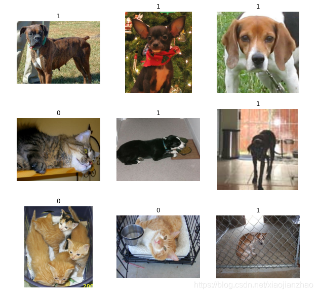
我们还可以看到标签1是“ dog”，标签0是“ cat”。

标准化数据

我们的原始图像有各种尺寸。另外，每个像素由0到255之间的3个整数值（RGB级别值）组成。这不适合提供神经网络。我们需要做两件事：

• 标准化为固定的图像尺寸。我们选择150x150。
• 标准化介于-1和1之间的像素值。我们将使用标准化层作为模型本身的一部分来进行此操作。
  通常，与采用已预处理数据的模型相反，开发以原始数据为输入的模型是一个好习惯。原因是，如果模型需要预处理的数据，则每次导出模型以在其他地方使用它（在Web浏览器中，在移动应用程序中）时，都需要重新实现完全相同的预处理管道。这很快就变得非常棘手。因此，在达到模型之前，我们应该进行尽可能少的预处理。

在这里，我们将在数据管道中进行图像大小调整（因为深度神经网络只能处理连续的数据批次），并且在创建模型时将其作为模型的一部分进行输入值缩放。

让我们将图像调整为150x150：

size = (150, 150)

train_ds = train_ds.map(lambda x, y: (tf.image.resize(x, size), y))
validation_ds = validation_ds.map(lambda x, y: (tf.image.resize(x, size), y))
test_ds = test_ds.map(lambda x, y: (tf.image.resize(x, size), y))

此外，让我们分批处理数据并使用缓存和预取来优化加载速度。

batch_size = 32

train_ds = train_ds.cache().batch(batch_size).prefetch(buffer_size=10)
validation_ds = validation_ds.cache().batch(batch_size).prefetch(buffer_size=10)
test_ds = test_ds.cache().batch(batch_size).prefetch(buffer_size=10)

使用随机数据扩充

当您没有大型图像数据集时，通过对训练图像进行随机但逼真的变换（例如随机水平翻转或小的随机旋转）来人为引入样本多样性是一种很好的做法。 这有助于使模型暴露于训练数据的不同方面，同时减慢过度拟合的速度。

from tensorflow import keras
from tensorflow.keras import layers

data_augmentation = keras.Sequential(
    [
        layers.experimental.preprocessing.RandomFlip("horizontal"),
        layers.experimental.preprocessing.RandomRotation(0.1),
    ]
)

让我们直观地看到经过各种随机转换后的第一批图像：

import numpy as np

for images, labels in train_ds.take(1):
    plt.figure(figsize=(10, 10))
    first_image = images[0]
    for i in range(9):
        ax = plt.subplot(3, 3, i + 1)
        augmented_image = data_augmentation(
            tf.expand_dims(first_image, 0), training=True
        )
        plt.imshow(augmented_image[0].numpy().astype("int32"))
        plt.title(int(labels[i]))
        plt.axis("off")

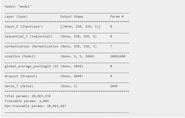
建立模型

现在让我们建立一个遵循我们先前解释的蓝图的模型。

注意：

• 我们添加了归一化层以将输入值（最初在[0，255]范围内）缩放到[-1，1]范围。
• 我们在分类层之前添加一个Dropout层，以进行正则化。
• 我们确保在调用基本模型时传递训练= False，以便它在推理模式下运行，以便即使在取消冻结基本模型以进行微调后，batchnorm统计信息也不会得到更新。

base_model = keras.applications.Xception(
    weights="imagenet",  # Load weights pre-trained on ImageNet.
    input_shape=(150, 150, 3),
    include_top=False,
)  # Do not include the ImageNet classifier at the top.

# Freeze the base_model
base_model.trainable = False

# Create new model on top
inputs = keras.Input(shape=(150, 150, 3))
x = data_augmentation(inputs)  # Apply random data augmentation

# Pre-trained Xception weights requires that input be normalized
# from (0, 255) to a range (-1., +1.), the normalization layer
# does the following, outputs = (inputs - mean) / sqrt(var)
norm_layer = keras.layers.experimental.preprocessing.Normalization()
mean = np.array([127.5] * 3)
var = mean ** 2
# Scale inputs to [-1, +1]
x = norm_layer(x)
norm_layer.set_weights([mean, var])

# The base model contains batchnorm layers. We want to keep them in inference mode
# when we unfreeze the base model for fine-tuning, so we make sure that the
# base_model is running in inference mode here.
x = base_model(x, training=False)
x = keras.layers.GlobalAveragePooling2D()(x)
x = keras.layers.Dropout(0.2)(x)  # Regularize with dropout
outputs = keras.layers.Dense(1)(x)
model = keras.Model(inputs, outputs)

model.summary()

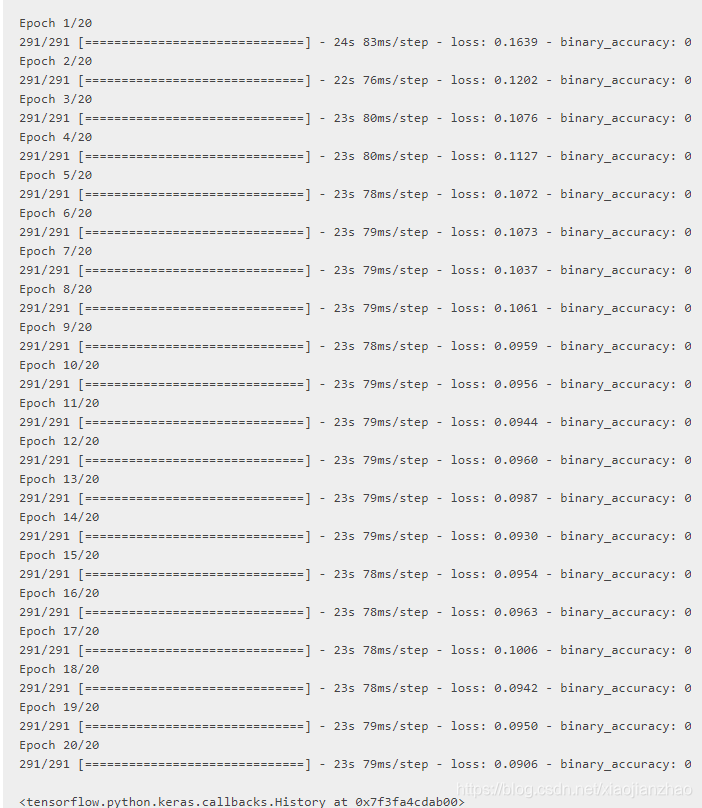
训练顶层

model.compile(
    optimizer=keras.optimizers.Adam(),
    loss=keras.losses.BinaryCrossentropy(from_logits=True),
    metrics=[keras.metrics.BinaryAccuracy()],
)

epochs = 20
model.fit(train_ds, epochs=epochs, validation_data=validation_ds)

对整个模型进行一轮微调

最后，让我们解冻基本模型并以较低的学习率端到端地训练整个模型。

重要的是，尽管基本模型变得可训练，但由于我们在构建模型时调用该模型时传递了training = False，因此它仍在推理模式下运行。 这意味着内部的批处理规范化层不会更新其批处理统计信息。 如果这样做的话，他们将破坏迄今为止该模型所学习的表示形式。

# Unfreeze the base_model. Note that it keeps running in inference mode
# since we passed `training=False` when calling it. This means that
# the batchnorm layers will not update their batch statistics.
# This prevents the batchnorm layers from undoing all the training
# we've done so far.
base_model.trainable = True
model.summary()

model.compile(
    optimizer=keras.optimizers.Adam(1e-5),  # Low learning rate
    loss=keras.losses.BinaryCrossentropy(from_logits=True),
    metrics=[keras.metrics.BinaryAccuracy()],
)

epochs = 10
model.fit(train_ds, epochs=epochs, validation_data=validation_ds)

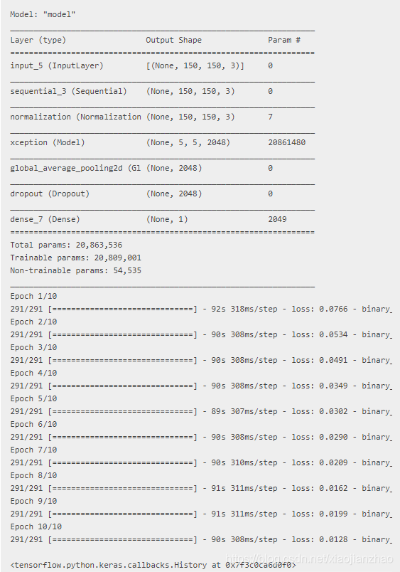
经过10个epoch后，微调在这里取得了很大的进步。

参考文献

• Transfer learning & fine-tuning